
WIPL-D Pro is an extremely powerful solver for fast and accurate electromagnetic analysis of arbitrary composite 3D metallic and dielectric structures.
The Numerical Engine
WIPL-D kernel has a set of unique features each contributing to unprecedented numerical efficiency. Along with unique features of full wave EM simulations goes the unique way in expressing the electrical size of a problem through a number of unknowns, rather than a number of mesh elements.
The numerical engine is based on the Method of Moments (MoM) SIE applied to quadrilateral mesh elements. Unlike some other numerical methods, where meshing of the entire volume occupied by the model is required, WIPL-D kernel meshes only the surfaces. One good side of this choice is that a model volume does not influence the size of the problem. For example, when simulating the coupling between two antennas, it is solely the size of the antennas that determines the size of the problem, not the distance between the two, and the number of unknowns remains the same with the changing distance. The other important consequence of meshing the model surfaces only is that no boundary box is required to artificially limit the model space. This is particularly important for open‑region problems, such as antenna design or antenna placement.
Comparing the quad mesh used in WIPL-D Pro with a triangular mesh used elsewhere, it is obvious that a number of the mesh elements is nearly halved with the quads, as each quad comprises two triangles. Accordingly, when using the same approximation technique, the number of unknowns is inherently about two time smaller with the quad mesh. However, the basis functions used on each element in WIPL-D are Higher Order Basis Functions (HOBFs) and Ultra Higher Order Basis Functions (UHOBFs) allowing for very large quads, as large as 2 by 2 wavelengths for HOBFs and 10 by 10 wavelengths for UHOBFs. Working with elements of such a large size significantly reduces a number of mesh elements on each surface further reducing the total number of unknowns several times.
A range of specially developed numerical techniques have been implemented in the kernel resulting in highly stabile computations. Due to the high numerical stability, it is possible to efficiently simulate models where extremely small mesh elements, measuring only a small fragment of a wavelength, are mixed with large mesh elements, measuring even a couple of wavelengths. A typical example of such a mixed arrangement could be the case of an antenna with electrically small details mounted onto a large metallic platform with a length in excess of dozens, or even hundreds of wavelengths.
Besides the unprecedented speed of the computations, high accuracy is equally important inherent property of WIPL-D kernel. There is no compromise between the speed and the accuracy as the latter have been confirmed via numerous benchmarks including the comparison with the measured data or with the results available in an analytical form. As the simulations are very efficient, for the cases where reliable comparison data are not available, a detailed convergence study can be carried out ensuring a high level of confidence for users with diverse level of EM simulation skills and experience.
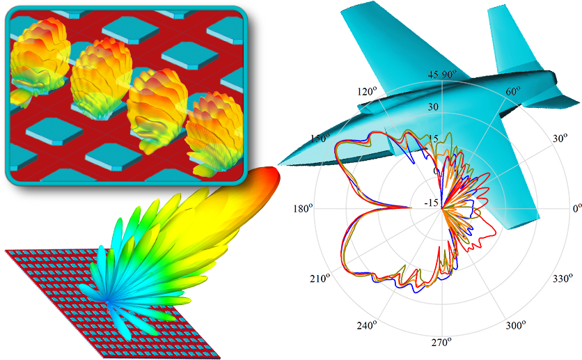
The result directly available after the simulations finishes is a distribution of currents over the surfaces. By default, for the case of an antenna or a microwave network, the kernel calculates Y, Z, and S parameters for the multiport described by the model. Near field distribution or far field radiation patterns can be calculated for the points specified by user. In addition, the calculated current distributions can be processed to obtain SAR, radiation pattern at finite distance, RCS at finite distance and numerous more advanced features.
To minimize the computational effort required for the cases where the calculations are very demanding, for example the calculation of the monostatic RCS, sophisticated interpolation algorithms were developed allowing the accurate interpolation between calculated response in frequency or radiation pattern points. It is even possible to interpolate current coefficients calculated over mesh elements.
The kernel can be executed on a variety of hardware platforms. Due to the quad mesh and HOBFs, even a standard machine, like an inexpensive everyday PC or a laptop, provides sufficient computational power to successfully solve electrically small and medium problems. When the problem requires the amount of memory exceeding the one installed on a machine, the efficient out-of-core solution method is used. The computation parallelization algorithms developed along with the WIPL-D kernel let the user take the full advantage of multi-core computers or platforms equipped with one or more GPU cards and significantly speed up the simulations. Utilization of GPU solver is essential when simulating electrically very large EM problems, where a number of unknowns is in the range of hundreds of thousands. Alternatively, when dealing with the problems of the same proportion, the parallelized kernel can be used on GPU clusters. Finally, for the most demanding problems, those requiring up to several millions of unknowns, DDS solver can be used.
Additional special computational techniques and advanced approximation features have been developed to support the efficient operation of the kernel for the case of electrically large structures. Namely Smart Reduction for Antenna Placement, Shadow Regions, Transparent Radome, Symmetry, Advanced Symmetry, or reducing a number of unknowns in the user-defined regions are all specifically targeting the reduction of a number of unknowns and consequently the simulation time for a number of practically important scenarios.
Development of some of the features listed have been driven by the customers interested to speed up computations related to a particular class of problems. Besides interacting with the WIPL-D development team and effectively streamlining the direction of the program evolution and improvement, a user is always welcomed to put to work the expertise, experience and dedication of the WIPL-D support team to make the most of the WIPL-D suite.
The short simulation time extends the possible application areas to those where a MoM solver is not commonly used. The first example can be the simulation of an ultrawideband (UWB) antenna or an UWB microwave circuit where a very large number of frequency points is required to reliably characterize the structure. Another fascinating example could be the fact that even the time-domain simulations with our Time Domain Solver, where Fourier transformation is used to convert the data from a large number of frequency points to time domain response, becomes feasible with WIPL-D MoM kernel. These multi-frequency problems could be additionally speeded-up by adjusting the number of unknowns as the operation frequency changes (the “freq” feature) or by simultaneously running multiple frequency points in parallel (on multicore or multi GPU systems).
Interface
With WIPL-D Pro, complex 3D models are created using wires, plates and predefined (meshed) 3D objects as building blocks. Drawing of the model using these objects actually defines the mesh that will be used during the simulation phase. In fact, a process of drawing the model is a process of defining the mesh. Therefore, when working with WIPL-D classics, the in-house developed model editor, the user is required, but in the same time allowed, to take the full control over the mesh, so the projects developed in WIPL-D pro usually have optimal number of unknowns resulting in minimal EM simulation requirements.
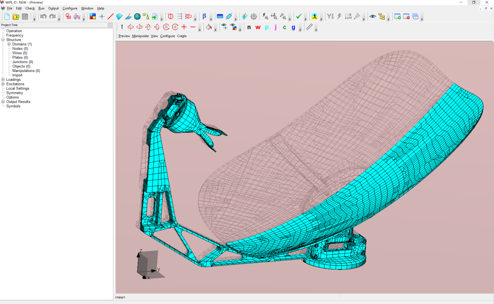
The Preview window provides a 3D isometric view of a model. All the entities used to define a model, such as node coordinates, wires, plates etc. are listed in tables or in the project tree. A model can be conveniently parametrized using symbolically declared variables via Symbol table. Unlike the meshing process in some other automated CAD tools, where the mesh phase is sometimes longer than the simulation itself, the parametrized mesh in WIPL-D Pro updates instantaneously during the parameter sweep or optimization. WIPL-D Pro can simulate a model meshed automatically from WIPL-D Pro CAD. A typical example would be meshed platform (such as aircraft, car or ship) where the parametrized antenna is imported and mounted.
Application areas
WIPL-D Pro can be successfully used for wide range of applications, but is especially well suited and provides significant advantages when analyzing:
- arbitrary shape 3D antennas and antenna arrays
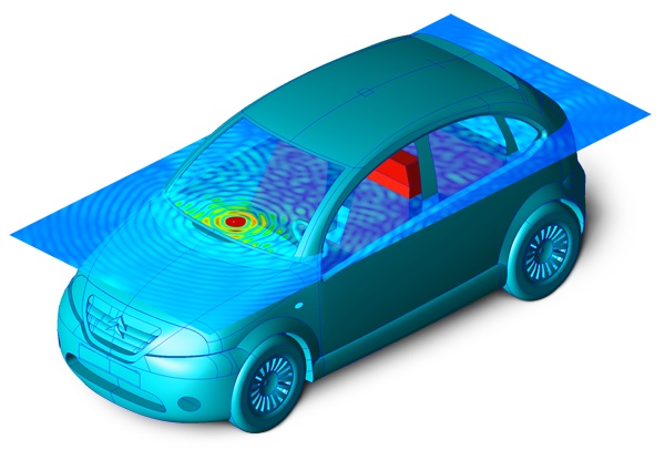
- large scatterers – vehicles, airplanes, boats, missiles
- antenna placement on large platforms
- transmission lines and waveguides
- microwave circuits over finite or infinite substrate
- metallic and/or dielectric scatterers of arbitrary shape
- EMC problems
- below kHz range applications

To get a feeling how WIPL-D can work to yours advantage please visit the Application area on our website, with special highlights on:
- Large reflector antennas
- Horn antennas
- Radomes
- Radar Cross Section (RCS) of large metallic platforms
- Antenna arrays
Get a free demo!