
 Similarly to the case of a GPU solver, which puts to good use the power of a GPU card to extend the performance of a single machine, GPU Cluster solver uses the power of the cluster computations to significantly speed-up the simulation and remarkably increase the size of a solvable problem, both far beyond the limits of a single machine. Cluster solver combines GPU and MPI parallelization using advanced algorithms and provides extreme versatility in operation as arbitrary number of compute nodes and arbitrary number of GPUs on each node can be used.
GPU Cluster solver is intended for fast solving of multi-frequency problems of medium or relatively large size on one side, and solving of electrically extremely large single-frequency problems on the other. In that sense, there are two operation modes of WIPL-D GPU Cluster Solver:
- Single-node solver – each cluster node simulates independent frequency samples or independent projects
- Multi frequency project is automatically divided into a number of single frequency projects, which are run in parallel on different cluster nodes
- Acceleration is proportional to the number of nodes
- Multi-node solver – multiple nodes are employed in solving of one problem
- All simulation steps (matrix fill-in, matrix inversion and post-processing) are executed one after another, each in parallel on all of the nodes employed
- The proportion of simulation time reduction is approximately equal to the number of nodes
- Maximum number of unknowns, which in most cases directly translates into maximum electrical size of the solvable problem, is significantly increased
Since each cluster configuration is unique, our solution is custom-made to best fit both, the available hardware and customer’s budget. For more info on our GPU cluster solution, please contact our Tech support.
Sample projects that were simulated on custom-made GPU cluster using the WIPL-D Cluster solver are presented below.
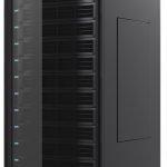
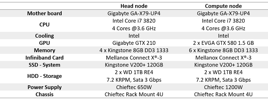 Configuration of the cluster used for the simulations
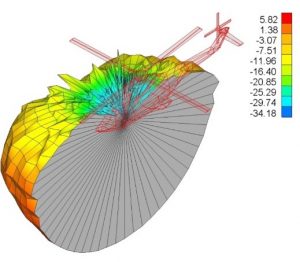
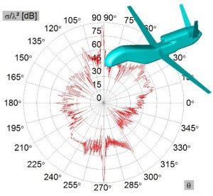 Example 1 – Monostatic RCS of global hawk
- Frequency of interest: 5 GHz
- Maximal dimension of the aircraft: 36 m (600 λ)
- Output results: monostatic RCS calculated in 1801 directions, in vertical plane
- One symmetry plane is used
- Number of unknowns: 546,000
- Simulation time (cluster with 8 nodes): 8 hours
Example 2 – Microstrip patch antenna at helicopter fuselage
- Frequency of interest: 2.7 GHz
- Helicopter length: 19 m (171 λ)
- Number of unknowns: ~404,253
- Simulation time (cluster with 6 nodes, each node has 2 GPUs): 7.7 hours